
 |
Tutorial: Data Analysis with Excel |
|---|
There are times when a best-fit line (ie, a first-order polynomial) is not enough. Calibration data that is obviously curved can often be fitted satisfactorily with a second- (or higher-) order polynomial. Calibration curves in atomic absorption are often slightly curved; here is an example from another tutorial.
You wish to analyze the lead concentration in tap water using graphite furnace AAS. The following data was collected. Report the concentration of lead in the tap water in the form of a confidence interval.
| lead conc, ppb | signal, A-s |
|---|---|
| blank | 0.006 |
| 10.0 | 0.077 |
| 20.0 | 0.138 |
| 30.0 | 0.199 |
| 40.0 | 0.253 |
| 50.0 | 0.309 |
| 60.0 | 0.356 |
| tap water sample | 0.278 |
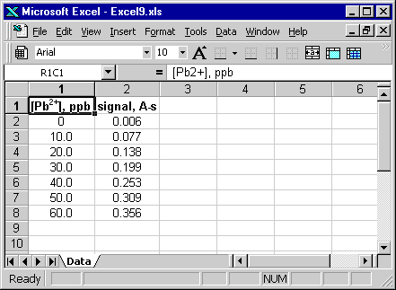
First the data must be entered into an Excel worksheet (click on image to download the file).
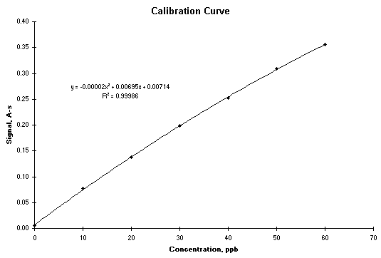
One way to perform polynomial regression is to fit the appropriate trendline to the data (and there are a number of options in addition to polynomials). The result is shown in the following screenshot.
 |
See how this is done. |
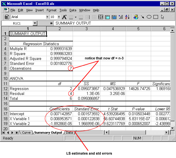
While the above approach is useful in providing additional information on a calibration plot, there is some information missing (such as the standard error in the estimates or the standard deviation in the residuals). It is possible to apply the Analysis ToolPak add-in to obtain this information. First, you must create another column whose cells contain the squared concentration values.
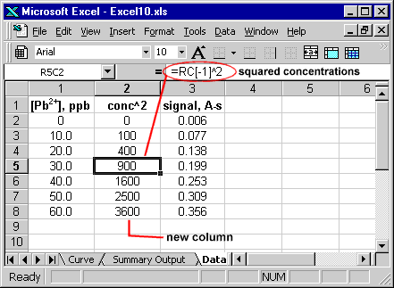
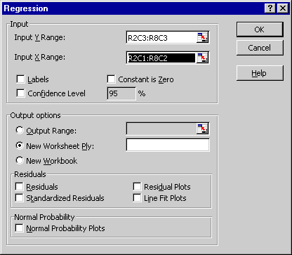
Now you can invoke the Analysis TookPak add-in. When choosing the X range, highlight the block that contains both the concentrations and their squared values.
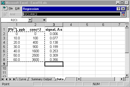
The regression dialog box should thus look like this:
The output of the regression module is shown below. Click on the image to download the Excel file.
 |
See a demonstration of how Analysis ToolPak is used to perform second-order polynomial regression |
 |