Linear Least-squares Regression in Excel

In the previous two Excel tutorials, we have discovered two ways to obtain least-squares estimates of the slope and intercept of a best-fit line:

• use the slope() and intercept() functions
• add a trendline to a scatterplot

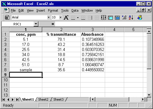
Both of these methods are quick and useful, but they are mere toys compared to the method outlined in this tutorial: using Excel's Analysis ToolPak add-in. Here is a screenshot of the calibration data (click to download the file):

First let's check that the add-in has been installed. Go to the Tools | Add-Ins sub-menu; you should see the following screen.

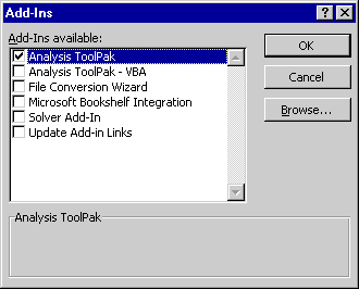
Make sure that the Analysis ToolPak is checked. Doing so will add a Data Analysis item to the Tools menu.

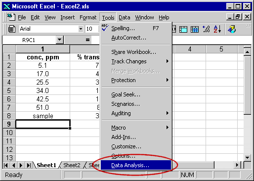
Select the Data Analysis item, and then scroll down and select Regression

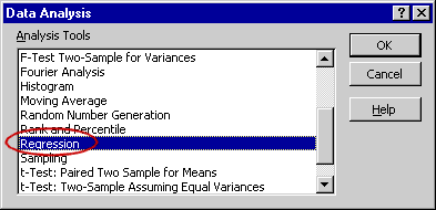
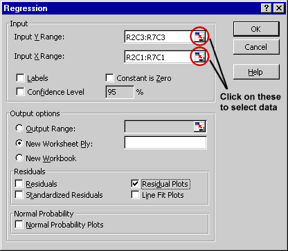
A dialog box will pop up. Select the ranges of the X and Y data; you can click on the funny little icons to select these ranges. It is also often a good idea to look at one of the residuals plots.

After clicking 'OK' a sheet will be created with statistical information about the linear regression.

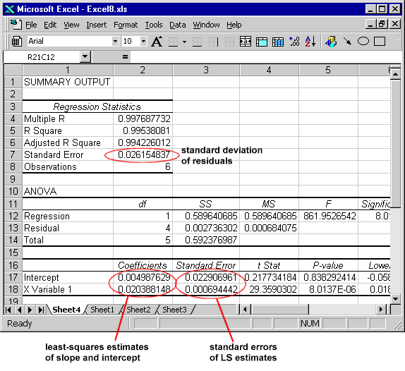
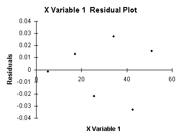
Click on the above image to download the Excel file. If you chose that particular option, a plot of the residuals will appear to help identify outliers and evaluate the appropriateness of the chosen regression model.

Watch the sequence of events leading to these last screen-shots