CHAPTER 5: LINKAGE I: BASIC EUKARYOTIC CHROMOSOME
MAPPING
I. Early evidence for
Linkage (the association of alleles of different genes on the same chromosome)
A. Bateson and Punnett early 20th century were working with sweet
peas with flower color and shape of pollen grains.
Using P = purple, p=red and L=long, and l=round
for pollen shape.
Crossed PPLL x ppll to get F1 dihybrid. Selfed
the dihybrid:
| |
Number of progeny in F2 |
| Pheno and geno type |
Observed |
Expected |
| Purple long (P-L-) |
4831 |
3911 |
| Purple round (P-ll) |
390 |
1303 |
| Red long (ppL-) |
393 |
1303 |
| Red round (ppll) |
1338 |
435 |
| total |
6952 |
6952 |
Found that a dihybrid cross did not give expected
ratios of 9:3:3:1
Nor did it look like any of the gene interactions
described in previous chapter.
What was unique was that the traits of the
parental generation appeared to influence the out come. PL and pl seemed somehow coupled
together.
Could see that a single gene followed Mendelian
ratios.
B. It took
T. H. Morgan to come up with explanation:
1.Using Drosophila genes:
Eye color: pr+ = red or pr = purple
Wing morphology: vg+ = normal wings or vg = vestigial wings
pr+ pr+ vg+vg+ x pr pr vg
vg
F1 pr+ pr vg+ vg
F2:
| phenotype |
Expected ratios |
Observed ratios |
| Red eyed normal wings
(pr+_ vg+_) |
9 |
>9 |
| Purple eyed normal
wings (pr_ vg+_) |
3 |
<3 |
| Red eyed vestigial
wings (pr+_ vg_) |
3 |
<3 |
| Purple eyed vestigial
wings (pr_ vg_) |
1 |
>1 |
2.Morgan test crossed the F1 female pr+ pr vg+ vg
with pr pr vg vg male. This allowed him to "see" how the genes from the
heterozygote female segregated because the male tester only contributes recessive alleles
| Male gametes |
pr vg |
| Female gametes (down) |
|
| pr+ vg+ |
pr+ pr vg+ vg |
| pr vg+ |
pr pr vg+ vg |
| pr+ vg |
pr+ pr vg vg |
| pr vg |
pr pr vg vg |
Progeny were:
| phenotype and genotype |
expected |
observed |
|
| Red eyed normal wings
(pr+pr vg+vg) |
0.25 |
0.47 |
parental |
| Purple eyed
normal wings (prpr vg+vg) |
0.25 |
0.054 |
nonparental |
| Red eyed vestigial
wings (pr+pr vgvg) |
0.25 |
0.053 |
nonparental |
| Purple eyed
vestigial wings (prpr vgvg) |
0.25 |
0.42 |
parental |
3. Morgan's observations
- 2 larger than expected classes carry the parental genotypes
- 2 smaller than expected classes carry the nonparental genotypes
- 1:1 ratio between the parental genotypes
- 1:1 ratio between the nonparental genotypes
Proposed the coupling of the dominant alleles PL
and the coupling of the recessive alleles pl
4. Next, he tried a cross for each
of the parents homozygous for one of the recessive alleles.
pr+ pr+ vg vg X pr pr vg+ vg+ ----> F1 pr+ pr
vg+ vg
test crossed F1 female pr+ pr vg+ vg X male pr pr vg vg
This allowed him to "see" how the genes from the heterozygote female segregated
because the male tester only contributes recessive alleles
| Male gametes |
pr vg |
| Female gametes (down) |
|
| pr+ vg+ |
pr+ pr vg+ vg |
| pr vg+ |
pr pr vg+ vg |
| pr+ vg |
pr+ pr vg vg |
| pr vg |
pr pr vg vg |
Progeny were:
| phenotype and genotype |
expected |
observed ratio |
|
| Red eyed normal wings
(pr+pr vg+vg) |
0.25 |
0.067 |
nonparental |
| Purple eyed
normal wings (prpr vg+vg) |
0.25 |
0.46 |
parental |
| Red eyed vestigial
wings (pr+pr vgvg) |
0.25 |
0.41 |
parental |
| Purple eyed
vestigial wings (prpr vgvg) |
0.25 |
0.063 |
nonparental |
Again, the ratios were not 1:1:1:1. In this case
the non allelic dominant genes appear to be repelling each other. Bateson and Punnett
called this situation repulsion.
5. Explanation of the larger than expected
classes that had the parental phenotypes.......T. H. Morgan's explanation was that the two
genes were on the same chromosome. This would explain their being together for most of the
progeny.
6. Explanation of the smaller than expected
classes that had the nonparental phenotypes.... To explain the two other smaller
classes, Morgan, using cytological evidence seen in the chiasmata seen at diplotene of
prophase I of meiosis, suggested that the chiasmata represent a breaking and reunion of
chromatids and a physical exchange of chromosome parts. These "recombined"
or recombinant chromosomes were responsible for the nonparental types.

(from An Introduction to Genetic Analysis, 6th ed. By Griffiths
et al. W. H. Freeman and Company)
7. Linkage can be in the coupling
(or cis) conformation where both recessive alleles are on the same chromosome of
the homologous pair or the repulsion (or trans) conformation where a
dominant allele of one gene is linked to a recessive allele of another gene.
8. Notation - when doing linkage problems
it is advisable to use the "Drosophila notation" where all the alleles from one
of the homologous chromosomes are written first followed by a slash and then the alleles
from the other member of the homologous pair are written. For example, for two genes
on chromosome #1 (A and B):
AB/AB x ab/ab ----> AB/ab
II. Recombination
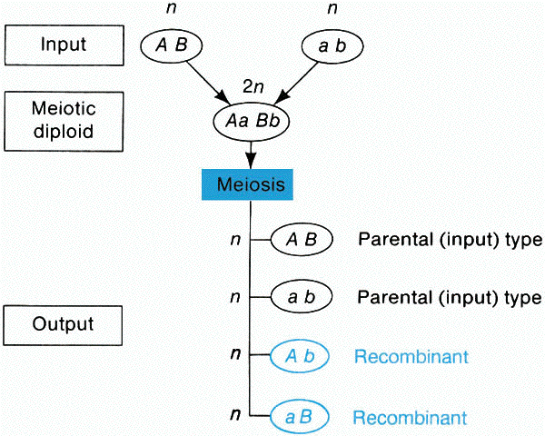
A. Meiotic recombination is any process that generates a haploid
product with a genotype that differs from both haploid genotypes that constituted the
meiotic diploid cell. Recombination is detected by comparing the output genotypes
with the input genotypes.

(from An Introduction to Genetic Analysis, 6th ed. By Griffiths
et al. W. H. Freeman and Company)
B.
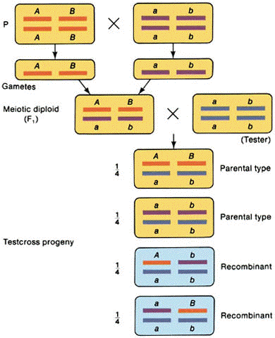
Interchromosomal recombination
1. Mendelian
independent assortment
2. A test cross yields 1 parental #1: 1 parental #2: 1 recombinant #1: 1 recombinant
#2
3. Occurs for genes on
separate chromosomes and genes that are very far apart on the same chromosome.

(from An Introduction to Genetic Analysis, 6th ed. By Griffiths
et al. W. H. Freeman and Company)
C. Intrachromosomal
recombination
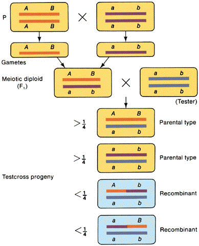
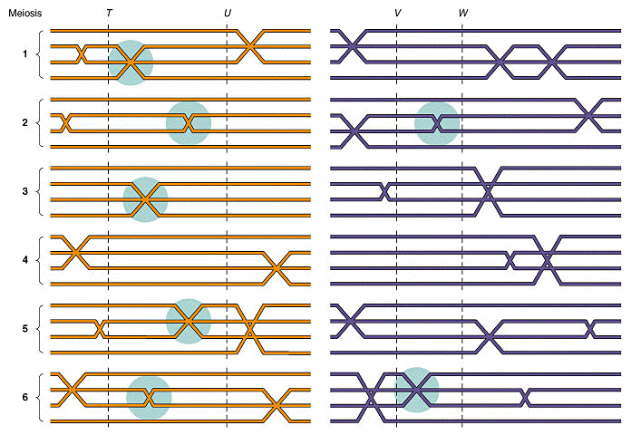
1. Recombination
generated by crossing over among nonsister chromatids of two homologous chromosomes.
2. Test cross
yields >25% parental #1: >25% parental #2: <25% recombinant #1: <25%
recombinant #2
3. Thus, a total
recombination frequency between two genes of <50% suggests that the genes are linked on
the same chromosome.
4. Cases where
recombinants are not recovered suggest that the genes are so tightly linked that they
never segregate.

(from An Introduction to Genetic Analysis, 6th ed. By Griffiths
et al. W. H. Freeman and Company)
III. Special cases of linkage on the X chromosome
For crosses that involve genes on the X chromosome, a homozygous recessive male can be
considered a tester strain because he only has one set of alleles to contribute.
Example of two linked genes on the X chromosome in
mice:
eye color gene: a+ for wild type and a for
apricot colored
coat color gene: g+ for for wildtype and g for grey colored
parental cross female wildtype (a+g+/a+g+)
X male apricot eyes and grey body (ag/Y)
F1 were wildtype females (a+g+/ag)
and wildtype males (a+g+/Y)
Selfed the F1 generation female a+g+/ag
X male a+g+/Y
| female gametes |
|
male gametes |
| a+g+ |
parental |
a+g+ |
| a+g |
recombinant |
| ag+ |
recombinant |
Y |
| ag |
parental |
F2 progeny (Notice that since the male progeny only inherit the Y chromosome from the
father, the female gametic contribution to the F2 males have no chance of being masked in
the male progeny. Thus, like a test cross, you can look at the frequency of each
phenotype in the male progeny to determine the frequency of the female gametes in the F1
generation)
| female |
male |
freq. |
|
| a+g+/a+g+ |
a+g+/Y |
>0.25 |
parental |
| a+g/a+g+ |
a+g/Y |
<0.25 |
recombinant |
| ag+/a+g+ |
ag+/Y |
<0.25 |
recombinant |
| ag/a+g+ |
ag/Y |
>0.25 |
parental |
IV. Linkage maps
A. Researchers had noticed that different recombination
frequencies were obtained between different linked genes. Morgan proposed that
differences in recombination frequencies were due to differences in the distances between
genes. Specifically,
the greater distance between two genes = greater the chance for recombination =
greater the recombination frequencies = less linkage

(from An Introduction to Genetic Analysis, 6th ed. By Griffiths
et al. W. H. Freeman and Company)
B. Morgan's student (Alfred Sturtevant) realized that
"variations in strength of linkage, already attributed ... to differences in spatial
separation of genes, offered the possibility of determining the sequences in the linear
dimension of a chromosome"
recombination frequency of 1% = 1 genetic map unit
(m.u.)
(100%)(# of recombinant progeny)/total # of progeny = # of genetic map
units
1. From the progeny of a dihybrid heterozygote test cross, we can
determine the distance between the two genes.
For example, the cross AB/AB x ab/ab is made ----> F1 = AB/ab
The F1 is backcrossed to the aabb parent (AB/ab x ab/ab)
The F2 are 2/6 AB/ab 1/6 Ab/ab 1/6 aB/ab 2/6 ab/ab
How far apart are A and B?
Parental gametes = AB and ab
Recombinant gametes = Ab and aB = 1/6 +1/6 = 2/6 = 0.33 or 33% or 33 map units
2. From a map distance between 2 genes, we can calculate the
expected progeny
For example the distance between A and B is 10 m.u.
What percent of the progeny will be AaBb in the cross AB/ab x ab/ab?
Parental gametes = AB and ab
Recombinant gametes = Ab + aB = 0.10
Thus, the freq. of the parental gametes = 0.90 and the freq. of each parental =
0.45 (AB = 0.45 and ab =0.45)
Thus, the freq of the AB/ab progeny will be 0.45 * 1 = 0.45
V. Three-point test crosses
The three point test cross is a test cross in which one parent is heterozygous for
three genes.
The steps for solving a three point test cross are:
1. assign parental genotypes (classes with the most progeny)
2. assign double recombinants (classes with the least progeny)
3. determine the gene order based on comparison of the parentals and the double
recombinants (the gene in the middle "flips" or
switches with respect to the other two flanking genes in the double crossover when
compared back to the parental)
4. rewrite the cross if needed
5. determine the frequency of single crossovers between genes A and B and genes B
and C (for the order ABC)
6. Draw map based on recombination frequency of 1% = 1 genetic map unit (m.u.)
For example, in Drosophila
eye color: v+ = wildtype and v =
vermilion eye color
wing veination: cv+ = wildtype and cv = crossveinless
wing morphology: ct+ = wildtype and ct = cut wing edge
Parental cross: crossveinless, cut winged (v+
cv ct /v+ cv ct) X vermilion (v cv+ ct+/v cv+ ct+)
F1 were triple heterozygotes (v+ cv ct/v cv+ ct+) wildtype
phenotype
Test cross: F1 wildtype (v+ cv ct/v cv+ ct+) X
triple mutant (v cv ct/v cv ct)
F2 progeny
| phenotype |
genotype |
# of progeny |
| v+ cv ct |
v+ cv ct / v cv ct |
592 |
| v cv+ ct+ |
v cv+ ct+ / v cv ct |
580 |
| v cv ct+ |
v cv ct+ / v cv ct |
45 |
| v+ cv+ ct |
v+ cv+ ct / v cv ct |
40 |
| v cv ct |
v cv ct / v cv ct |
89 |
| v+ cv+ ct+ |
v+ cv+ ct+ / v cv ct |
94 |
| v cv+ ct |
v cv+ ct / v cv ct |
3 |
| v+ cv ct+ |
v+ cv ct+ / v cv ct |
5 |
|
|
1448 |
1. Parental phenotypes are the most numerous classes = v+ cv ct and v cv+ ct+
2. Double crossovers are the least numerous classes = v cv+ ct and v+ cv ct+
3. Determination of the gene order by comparison of
the parental and double cross over classes (the gene in the middle "flips" or
switches with respect to the other two flanking genes in the double crossover when
compared back to the parental): so in this case, the gene order is v ct cv
4. Rewrite the crosses:
Parental cross: crossveinless, cut winged (v+ ct
cv /v+ ct cv) X vermilion (v ct+ cv+/v ct+ cv+)
F1 were triple heterozygotes (v+ ct cv/v ct+ cv+) wildtype phenotype
as F1 wildtype (v+ ct cv/v ct+ cv+ ) X triple mutant (v
ct cv/v ct cv)
5a. Determine the frequency of crossover between the
v and ct loci:
Parentals are v+ ct and v ct+ and recombinants are v+ct+ and v ct
(89+94+3+5)/1448 = 0.132 = 13.2% = 13.2 m.u.
5b. Determine the frequency of crossover between the
ct and cv loci:
Parentals are ct cv and ct+cv+ and recombinants are ct cv+ and ct+ cv
(45+40+3+5)/1448 = 0.064 = 6.4% = 6.4 m.u.
6. Thus the map is
| v__________________________ |
ct________________ |
cv |
| 13.2m.u. |
6.2m.u. |
|
VI. Interference
Interference is the measure is the independence of crossovers from each other.
Interference (I) = 1- the coefficient of coincidence (c.o.c)
The coefficient of coincidence (c.o.c) is the ratio of the observed number of double
recombinants to the expected number of double recombinants (observed # of double
recombinants/expected # of double recombinants OR
observed frequency of double recombinants/expected frequency of double
recombinants).
Thus, I = 1 - (observed # of double recombinants/expected # of double
recombinants)
If I = 1, the double crossover event never occurs. If I = 0, there is
no interference.
Consider the above three point test cross as an example.
The expected number of double recombinants = the probability of a single crossover between
the v and ct loci * the probability of a single crossover between the ct and cv loci*total
# of progeny
Expected doubles = (0.132)(0.064)(1448) = 12
I = 1 - (5+3/12) = 0.33
VII. Calculating recombination frequencies from selfed dihybrids:
The three point testcross is the best way to examine linkage; however, many times a
double recessive homozygote tester is not available. Recombination frequencies can
be calculated from selfed heterozygous dihybrids (although the frequencies obtained are
not as exact as a test cross because of the mathematical manipulations involved).
Consider two genes A and B
Parental cross AB/AB X ab/ab
F1 = AB/ab
Self the F1 AB/ab X AB/ab
| F2 Genotype |
# of F2 progeny |
| A-B- |
284 |
| A-bb |
21 |
| aaB- |
21 |
| aabb |
55 |
| |
381 |
In this cross, the only complete genotype that we know is aabb (ab/ab) which occurs at
a frequency of 55/381 = 0.144
We know that ab/ab resulted from male ab gamete fusing with female ab gamete and that the
frequency of these gametes being produced is equal in the male and the female since they
are both F1s.
So let a = frequency (or probability) of the ab gamete forming.
P(ab from male)*P(ab from female) = 0.144
a*a = 0.144
a2 = 0.144
square root of a = square root of 0.144
a = 0.3799
ab and AB are both parentals and will form at the same frequency which we just
calculated to be 0.3799
Thus, the total frequency of the parentals = freq. of ab + freq. of AB = 0.3799 +0.3799 =
0.7598
If the freq. of the parentals = 0.7598, then the frequency of the recombinants = 1 -
0.7598 = 0.2402
Thus the recombination freq. = 24.02% = and the genes are 24.02 m.u. apart
Lecture
Syllabus Page | Home Page
This web site created and
maintained by Dr. Laura Runyen-Janecky
Last updated on 19 Jul 1999

