![\includegraphics[height=1.5in]{f1.eps}](img98.png)
where the
I pledge that I have given nor received unauthorized assistance during the completion of this work.
Signature: width10cm height1pt depth0pt
Questions (3 pts. apiece) Answer questions in complete, well-written sentences WITHIN the spaces provided.
Problems. Clearly show all work for full credit.
| 1. (8 pts.) |
The work function of zinc is 3.6 eV. What is the energy of the most energetic photoelectron
emitted by ultraviolet light of wavelength 2400 |
| 2. (17 pts) |
At 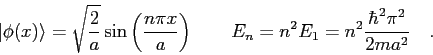
|
| 3. (17 pts) |
Find Make sure you get an expression for
|
Continue ![]()
Problems (continued). Clearly show all work for full credit.
| 4. (17 pts) |
In the phenomenon of cold emission, electrons are drawn from a metal at room temperature
by an externally supported electric field.
The potential well the metal presents to the free electrons before the electric field is turned on
is shown in Figure 1a below.
After application of the constant electric field
where
|
Continue ![]()
Problems (continued). Clearly show all work for full credit.
| 5. (17 pts) |
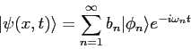
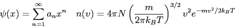
In solving the Schroedinger equation for the harmonic oscillator
potential we rewrote the Schroedinger equation
in the form
where  .
We then showed the asymptotic solution is .
We then showed the asymptotic solution is
We then made the guess that the initial wave function will be of the form where 
where |
The wave function,
![]() , contains all we know of a system and
its
square is the probability of finding the system in the region
, contains all we know of a system and
its
square is the probability of finding the system in the region ![]() to
to
![]() .
The wave function and its derivative are (1) finite, (2)
continuous, and (3) single-valued.
.
The wave function and its derivative are (1) finite, (2)
continuous, and (3) single-valued.


![\begin{displaymath}
\overline K = {3\over 2} kT \quad
\zeta_1 = {\bf t}\zeta_3 =...
..._{x_0}^{x_1}
\sqrt {2m(V(x) - E) \over \hbar^2} ~ dx\right ]
\end{displaymath}](img55.png)

|
Speed of light ( |
|
fermi ( |
|
|
Boltzmann constant ( |
|
angstrom ( |
|
|
|
electron-volt ( |
|
|
|
Planck constant ( |
|
MeV | |
|
|
GeV | |
|
|
Planck constant ( |
|
Electron charge ( |
|
|
|
|
|
|
|
Planck constant ( |
|
Electron mass ( |
|
|
|
|
||
|
Proton mass ( |
|
atomic mass unit ( |
|
| |
|
||
|
Neutron mass ( |
|
Avogadro's Number |
|
| |
( |
![\includegraphics[width=5.5in]{periodic_chart2.eps}](img97.png)
![\includegraphics[height=1.0in]{p2a.eps}](img29.png)
![\includegraphics[height=1.5in]{p2b.eps}](img30.png)